2013-04-29

Remaining tests

1. Nightly science stack test/comparison.
2. skycell.027 y-filter 2009 data only (this is the data that fills in the high-variance region).

2013-04-26

Deep stack comparison

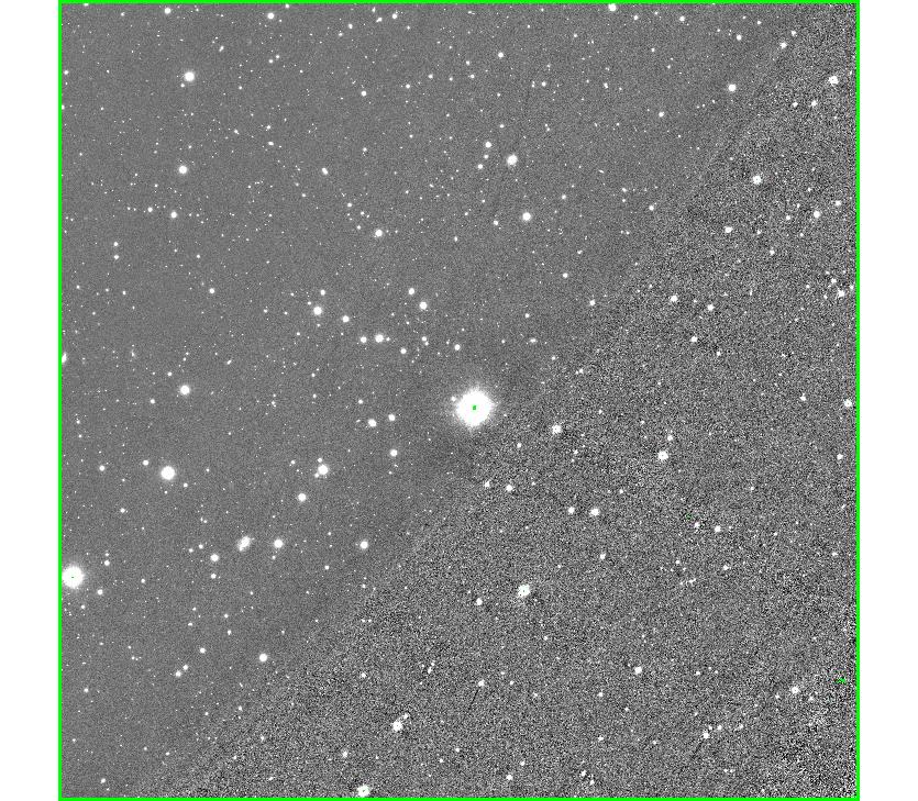
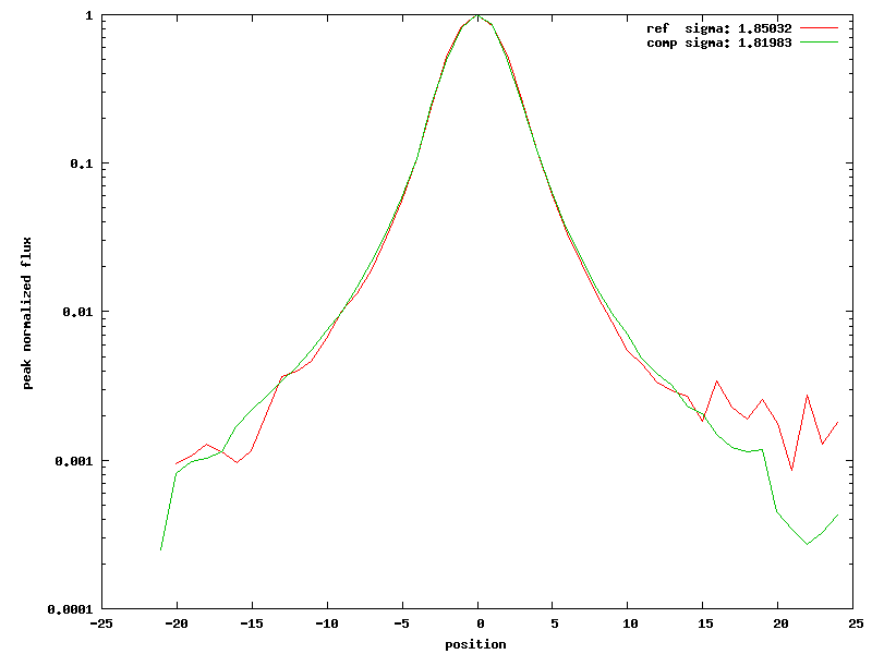
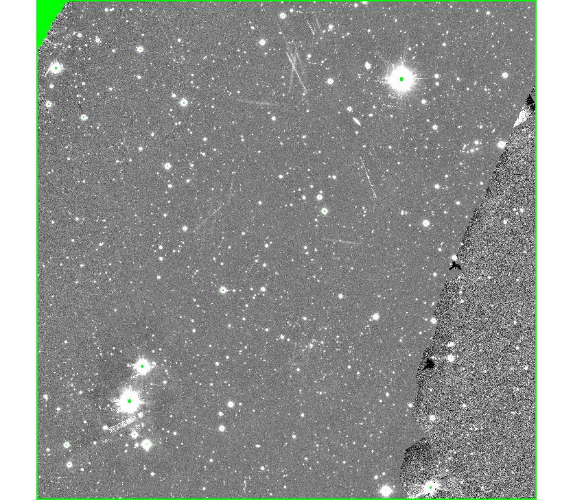
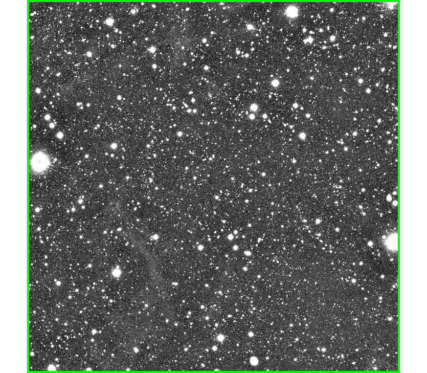
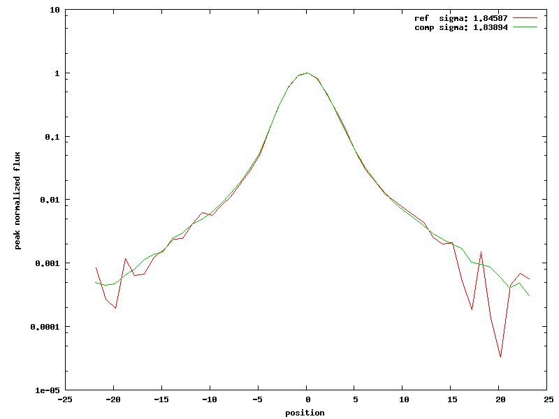
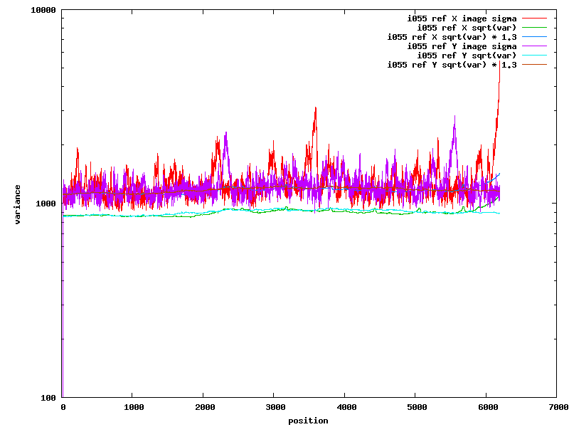
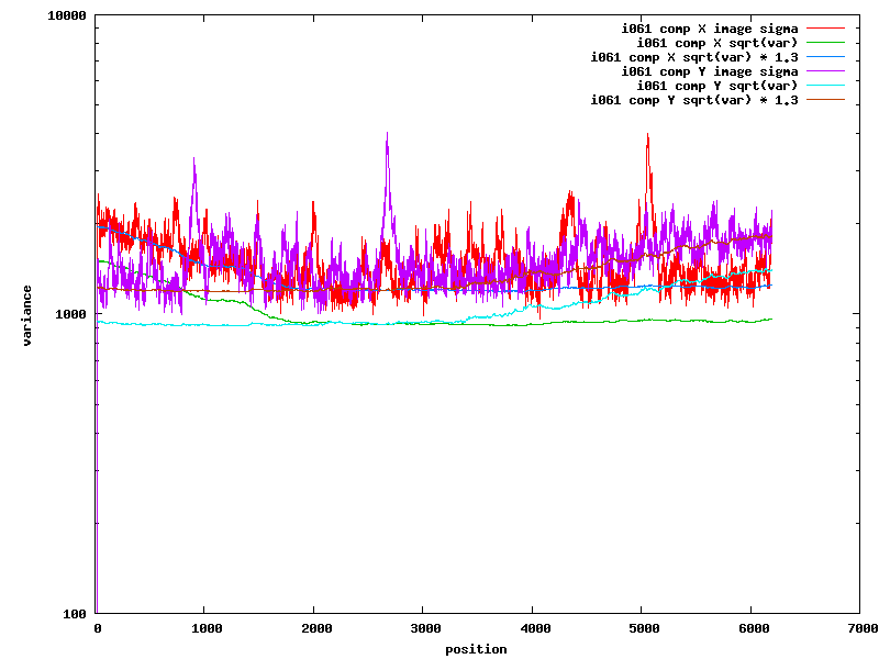
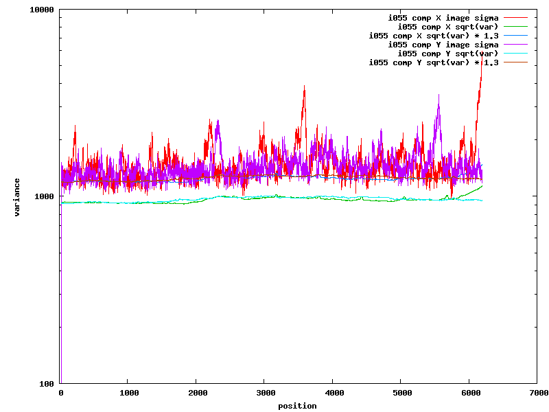
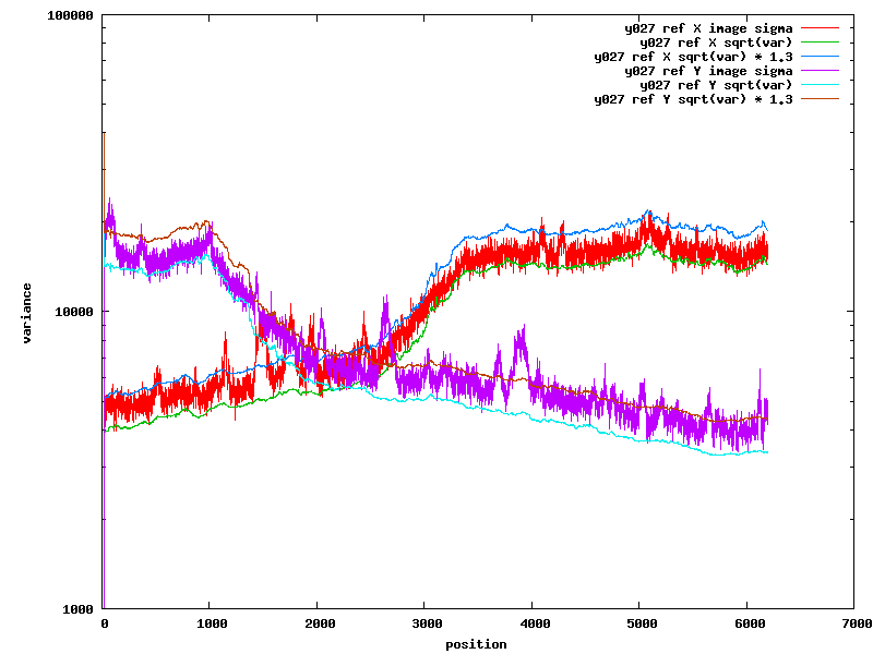
The following table shows the comparison between the current MD09 deep stacks (deeptest) and the reduction with the current ppStack changes (MDtest or comparison below). I used four skycells that Mark noted were particular bad. The images show that the new code does a better job retaining images and that cleans up some of the i-filter skycell issues. However, this improvement does not extend to y/027, which still has a clear region of high variance. The profiles in the next column show a slice across the image from 2000-2500pixels in X (red) and Y (blue). The median variance for that profile from the weight image is also displayed (in green and purple). This illustrates that the new reduction does remove some of the un-modeled image variance jumps that were present in i/041 and i/061. The final column shows the profile of a star in the stack for both the deeptest (red) and comparison (green) stacks, along with the Gaussian fit sigma value for each. These profiles suggest that even though the comparison target PSF is larger than in the deeptest stacks, the stellar profiles in the unconvolved stack do not change significantly.

It should be clear that the deeptest is not a reference stack used for difference images, nor is it an absolute deep stack. It was constructed as a test for examining the results of stacking large numbers of inputs in ppStack. However, there is no other stack available for these skycells that have comparable or greater coverage, and so it is used as the basis to compare the set of ppStack changes used in the MDtest stacks.

ID	label/reduction	inputs	accepted	Target FWHM	unconv image	data/variance profiles	stellar psf comparison
skycell.027 y	MD09.deeptest.20120727	187	133	10.321
	MDtest.20130425	299	207	8.626
skycell.055 i	deeptest	372	294	7.936
	MDtest	465	427	9.556
skycell.041 i	deeptest	339	167	6.598
	MDtest	423	359	9.863
skycell.061 i	deeptest	356	72	6.681
	MDtest	445	396	8.993

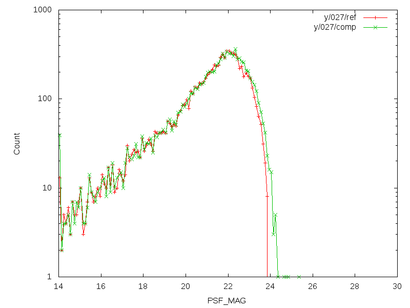
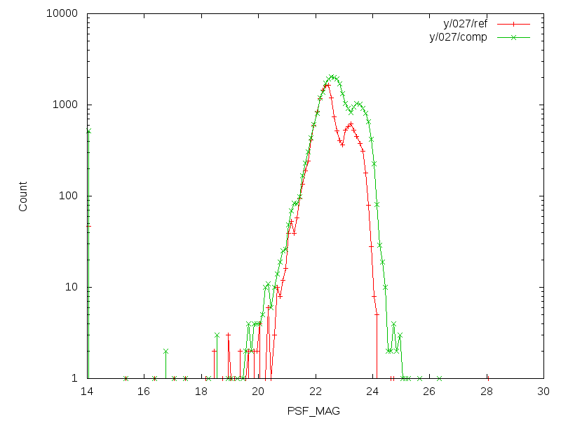
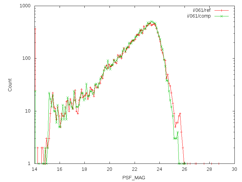
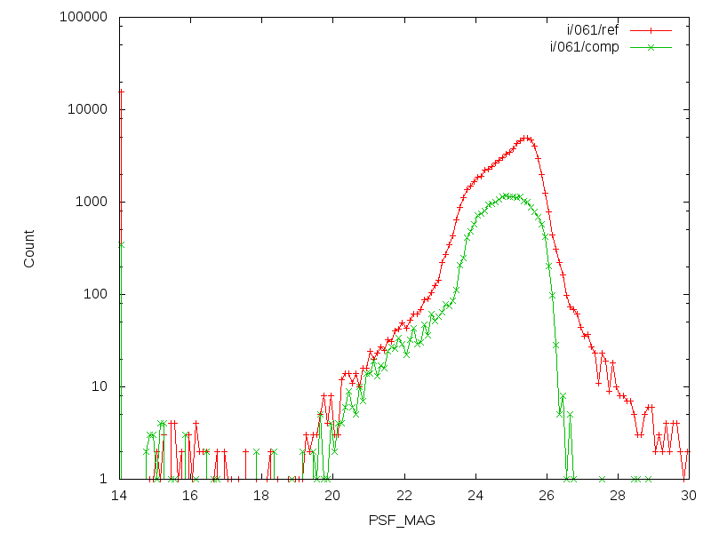
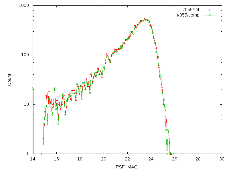
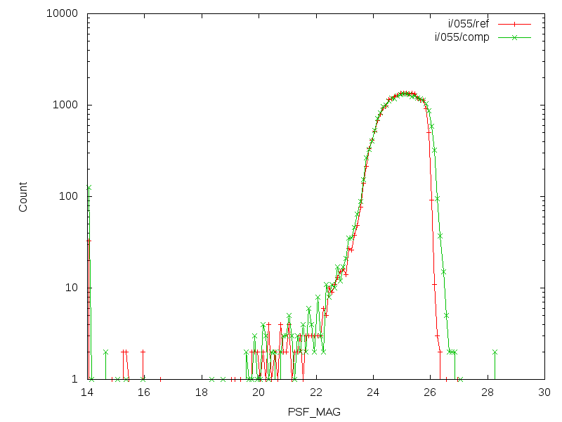
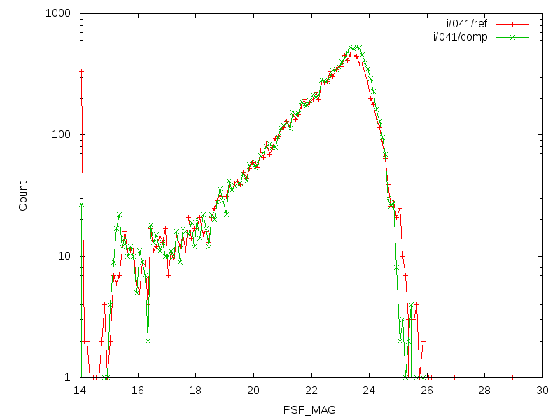
False positives: I matched the detection list from running psphot on the unconvolved stacks against a set of SDSS stripe 82 sources (constructed by Nigel). I then declared all unmatched detections as false positives, and plotted the magnitude distribution of those as well as all objects with those detections subtracted. This does set a detection limit based on the SDSS data. However, the new stacks generally have fewer unmatched detections than the previous, especially in the two fields that had bad combinations in the previous stacks.

field	False Positives	All detections - FP
skycell.027 y
skycell.055 i
skycell.041 i
skycell.061 i

2013-04-24

Conclusion

I believe the unrestricted reduction is the one we accept. There is an increase in the target PSF FWHM relative to the stricter standard reduction, although it is not significantly worse than the current analysis. There is a gain in image depth in some areas, and that translates into higher S/N for the majority of objects.

The only remaining test I would like to do is to process a deep stack that has difficulties with the target PSF to determine if these changes help those stacks as well. Optimally, if that deep stack is subjected to the excess detection bug, this deep stack test could evaluate both simultaneously.

Tests

The following images review the statistics for the SAS g.00000 data in four processings:

• SAS_v8. This is the current public release version of SAS, and was generated on 2012-07-19 22:32:40 with software_ver 34160.
• SAS123.ipp. This is a reprocessing of SAS using the current IPP tag (2013-04-19 23:59:00 with software_ver 35266). This is taken as the default against which the others are measured.
• standard. This is the initial proposed set of stacking changes, including SAFE=F, circularization fix, and bimodal input rejection. (2013-04-24 03:41:11/35307M)
• unrestricted. This is identical to the standard reduction above, but sets the minimum input threshold to 10.0pxl (only inputs above that are rejected with the bimodal code). (2013-04-24 03:41:11/35307M)

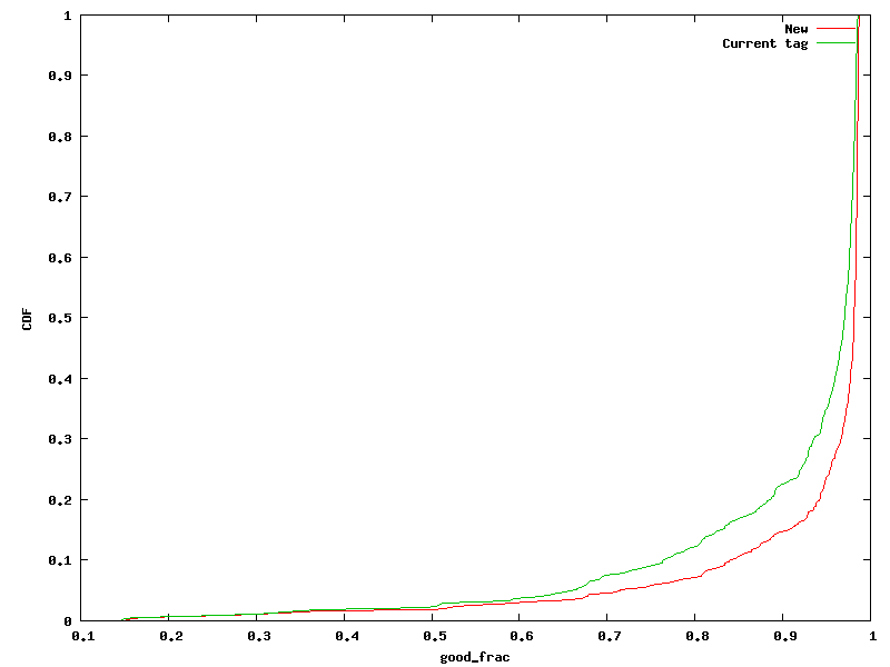
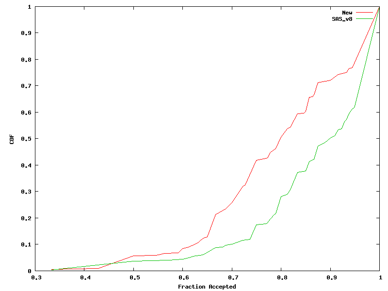
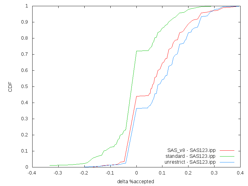
First, fraction of input images accepted into the stack (positive good). The SAS_v8 reduction had no input clipping, and so all excluded inputs are rejected at the PSF matching phase. The proposed standard reduction is somewhat more aggressive than the current tag, likely as a result of the "year 3" data having slightly different seeing than the "year 1+2" data. This induces a bimodality that the rejection code picks up on. The unrestricted reduction is more inclusive of things with slightly larger sizes, and due to the fixes in the chi^2 matching, excludes fewer images than the SAS_v8.

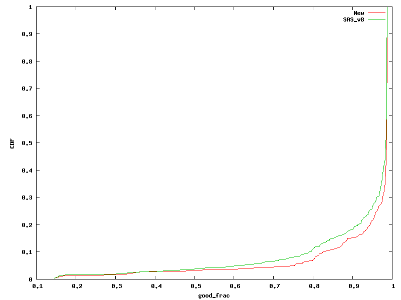
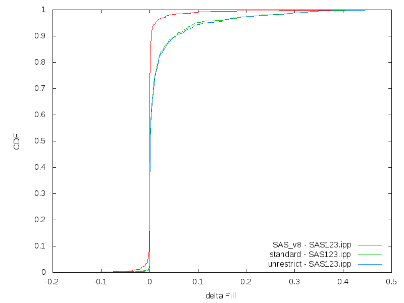
Fill factor (positive good) is not very surprising. Turning safety off results in much better fill factors compared with the previous reductions.

The .num files (positive good) contain the number of input images that contributed to a given pixel. This is largely a reflection of the acceptance plot above, showing that as we exclude more input images, the average contributions to a given pixel drops. The unrestricted reduction offers a median improvement of about 0.4 inputs/pixel, with the other reductions having little change.

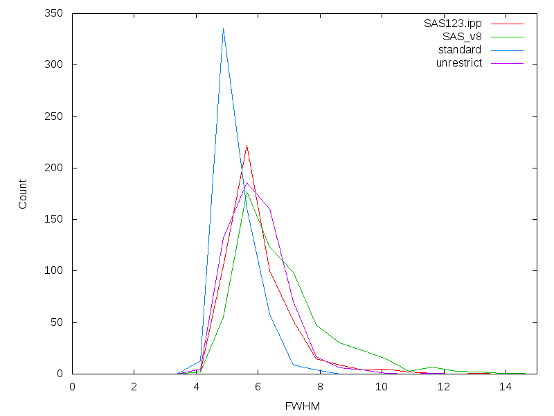
The above data suggests that switching to the unrestricted option (which will only clip the worst outliers) is probably a good idea. The concern for this is that we will increase the size of the target PSF. Correcting the circularization bug seems to help constrain the targets reasonably well. The SAS_v8 reduction did not have this correction, and did not restrict any inputs, and has the largest PSF size. The standard reduction clips strongly to keep the target PSF size down, and as such, does not increase it relative to the current tag. The unrestricted PSFs are larger than the current tag, but looking at the histogram of FWHM values, it does not seem to push to extreme values, with nearly all targets smaller than 8pxl.

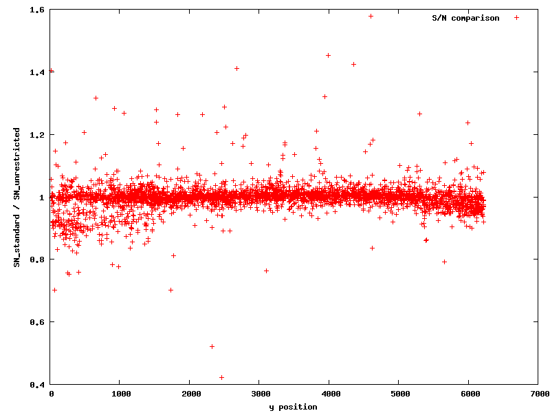
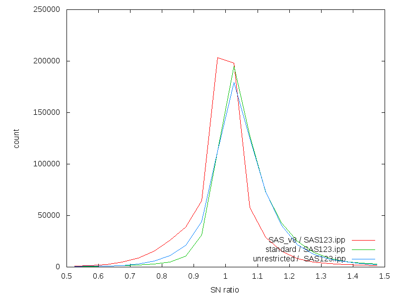
Checking the S/N values for detections in the stack CMF files (so there is no reanalysis of the images in this plot. Only previously known objects are photometered) shows that there is an improvement in the S/N compared to the current tag:

2013-04-23

The circularization bug appears to be a result of an issue in the pmPSF_AxesToModel and pmPSF_ModelToAxes functions that resulted in a factor of ~2 error in the sizes. With this bug resolved, the Target PSF for the example below drops to 4.815245 pxl. Removing any restriction on the input FWHM sizes (-Df PSF.INPUT.THRESH 10.0 so all inputs with FWHM < 10 are accepted) produces a target PSF of 6.571348. As even this is a factor of 2 smaller than the target PSF created before the bug fix, I'm beginning to suspect that we may have been aggressively clipping the inputs as a result of this bug.

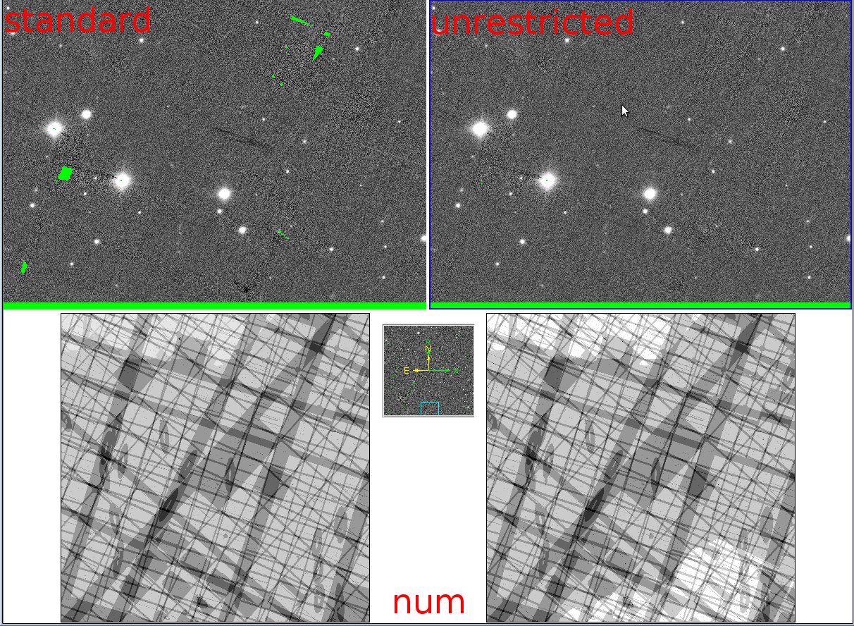
The two metrics that are most likely to clarify whether a given stacking recipe is better than another are the average value of the .num image produced (the average number of inputs for a given pixel in the stack) and the S/N distribution of detected objects. For the initial test, I've run the rejection I've been developing (the standard recipe), along with the rejection with PSF.INPUT.THRESH set to 10.0 (the unrestricted recipe). The following image shows the number image on the bottom row, along with a zoom in of a section of the unconvolved image (with finding chart displayed). In the region of this zoom, the additional inputs that are not rejected at input (and have therefore survived the PSF matching phase as well) seem to help fill in gaps and correct some defects (dark spot, bottom middle of image; linear feature, middle right of image). Below this is a plot of the ratio of S/N values for all objects detected by psphot on these images as a function of y-position. As the change in depth is largely a function of y-position, this shows the difference. Note that at y < 1500pxl, the S/N ratio bifurcates, with the samples from areas of added inputs yielding a higher S/N (largely consistent with an improvement of 2 inputs: sqrt(8)/sqrt(10) ~ 0.9). The scatter in the S/N ratio increases at high y, correlating with the other region of increased depth.

This test suggests that restricting inputs based on FWHM may have been necessary due to a bug in the circularization process, and may no longer be needed. The follow-up test will be to measure these two metrics for the sample of:

• Stacks created with current IPP tag.
• Stacks created with proposed "standard" recipe, that does exclude inputs based on FWHM.
• Stacks created with proposed "unrestricted" recipe, that sets the input threshold at 10.0.

2013-04-22

Circularization

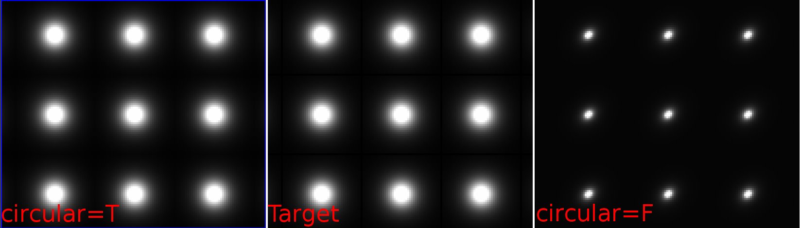
When ppStack generates a target PSF, it does so by taking the envelope of a "circularized" realization of the input PSFs. This appears to work fine for PSFs that are already circular, but for highly elliptical PSFs, this breaks down for unknown reasons. As an example, the following figure shows the PSF grid for input 14 for a certain SAS stack. The target grid shown in the middle is dominated by the large size of input 14. However, disabling circularization creates the field shown in the right panel. The circularized form seems much larger than expected from this elongated PSF. Looking at the profiles along the major and minor axis and comparing this to the circularized form shows that there is an error somewhere in this calculation.

The effect of this circularization error is that the input PSF cuts work on a PSF radial profile corresponding to the elliptical form. This produces a FWHM on the order of 4. This is below the threshold, and is therefore accepted. However, upon circularization, the FWHM balloons to ~11, resulting in a target PSF of ~11. This likely explains some of the unexpected jumps in target FWHM from a "well behaved" set of inputs.

Armin's questions/points

• Q1: "One good test to see if everything is propagated correctly is to check the noise"
• A1: I chose six horizontal stripes across the image, and calculated the image noise and variance median for each 100-pixel tall sample (partially because I have that code done and easy to use). To remove the effects of stars (which appear as horizontal excursions in the following plot), I used the median absolute deviation as the image noise statistic, converted in the plot to a Gaussian sigma. The variance image was measured using a simple median. No covariance term was applied, although a quick by-eye estimate suggests a covariance term of ~1.1. Each horizontal stripe sample is offset from the previous by 200 counts on both axes to reduce the confusion of overlaps.

• Q2: "If you look at the data, it is clear that for low flux, the X2 levels out at a constant value, and for large flux value it increases. This means that c1=0.0"
• A2: Agreed. Some consideration was made to switch to fitting a chi^2 floor with an exponential rise with flux, but that should yield effectively the same result as the log-log fit used.
• Q3: "What kind of errors do you assume when you fit stamp_chisqr versus stamp_flux?"
• A3: We use no errors on this fit, so they are implicitly weighted equivalently. This is certainly why the fit is biased when low-flux/high chi^2 points are included (such as in fit 0 here stacking_coverage.20130307). The quick answer would be to use Poissonian error estimates, which would reduce the weight of these outliers. I think the log-log fits reduce the weights of these outliers more (log10(~200)/log10(~30) < sqrt(~200)/sqrt(~30)).

2013-04-19

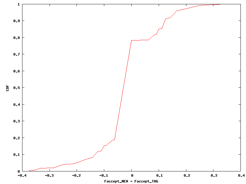
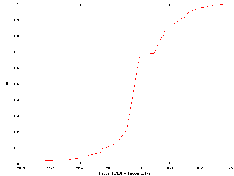
Comparison of SAS processing with current tag and with proposed updates. The first two columns show the apples-to-apples comparison of the current IPP tag and the proposed changes to the trunk. This shows that the improvement in the input rejection is roughly equal in the two versions of the code, with the SAS123 showing a slight favor to the proposed changes (30% improved input fraction compared with 20% that did not). The increase in the fill factor is largely a result of switching the safety flag to false, and not due to the increase in input number. The final column shows the comparison between the proposed changes and the original SAS_v8 processing from 2012-07-19. This processing did not have the stack input filtering enabled to the degree it currently is, and as a result, only failures in the PSF-matching phase contribute to the input rejection. Without this filtering, the fraction of inputs used is obviously higher. This raises the question of whether input filtering is really helpful for 3pi stacks.

	SAS12 tag vs proposed	SAS123 tag vs proposed	SAS123 SAS_v8 vs proposed
Fill factor
Fraction of inputs accepted
Difference in input fraction

2013-04-16 A

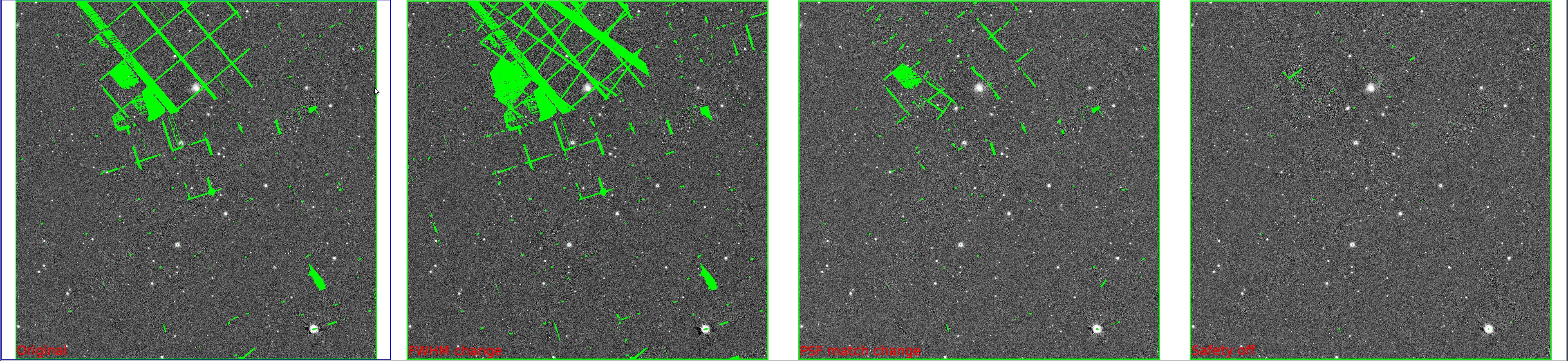
I was able to track down the quadratic fit problem as a result of fitting data with outliers that span many orders of magnitude. I put together a quick hack by taking the logarithm of the chi^2 and flux values, and fitting the quadratic to that. This greatly reduces the scatter found, and provides better fits to the actual data. The following comparison image shows the original stack combination, the reduction with the improved input FWHM cuts (which introduced the chi^2 cut issue), the reduction with this logarithm hack, and finally a result with all of the previous improvements but now with SAFE = F.

2013-04-16

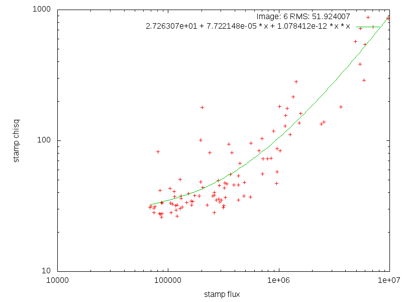
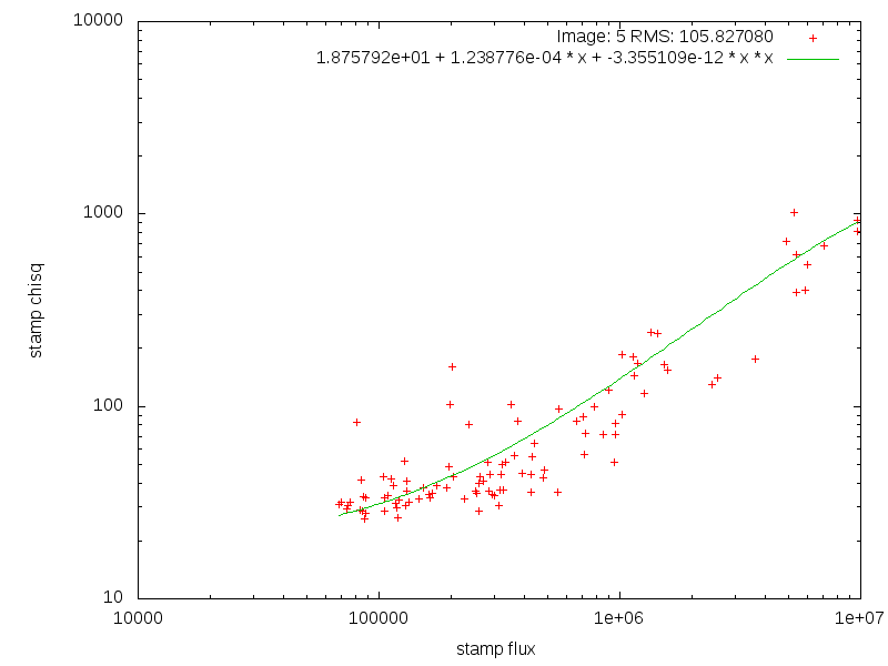
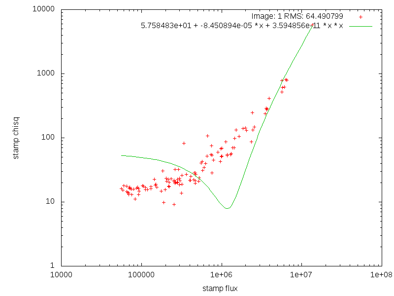
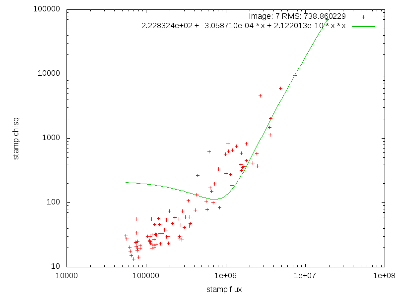
While testing the input FWHM cut, I discovered that an image that appeared valid by eye was being flagged during the PSF matching stage as having a overly deviant chi^2 value. A study of the code revealed that the chi^2 value used is calculated in the following way:

1. For all valid stamps in the PSF match, the flux and squared residual are fit with a quadratic function (x0 + x1 * flux + x2 * flux^2).
2. This quadratic function is subtracted from the squared residual, providing a flux-neutral measurement of the squared residuals.
3. The RMS scatter of these remaining residuals is saved as the chi^2 value for the PSF match (there's a sum over all used kernels, but the example case has only a single kernel).

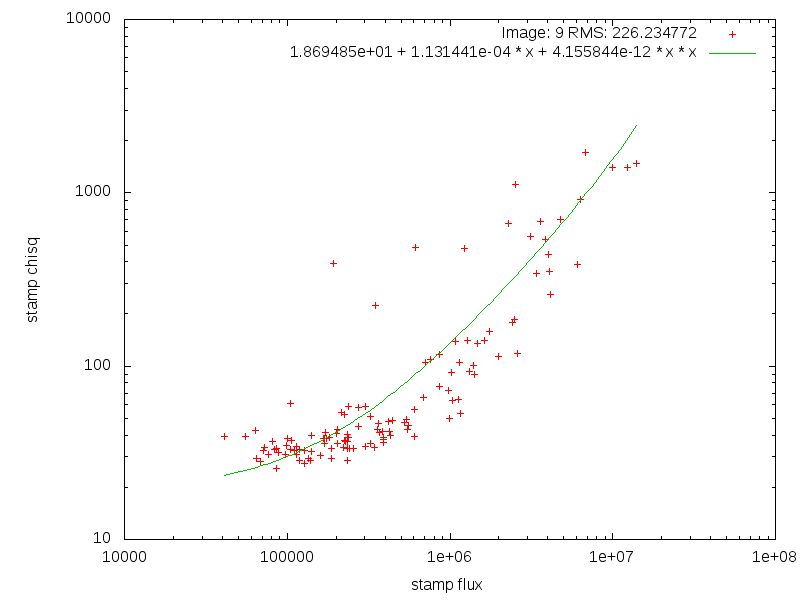
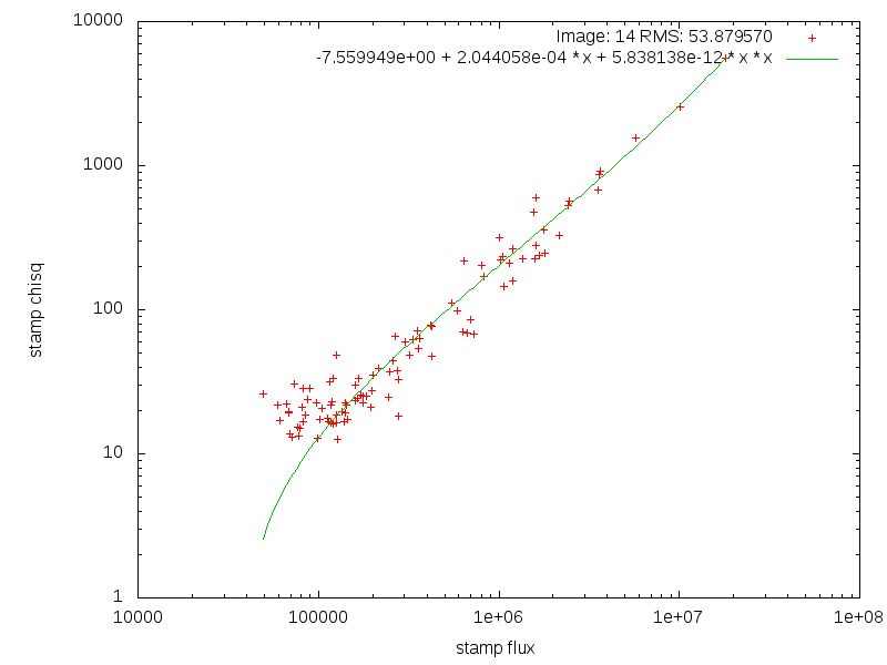
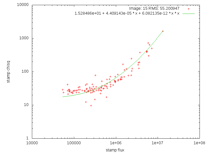
The following table shows the set of PSF match values, along with the parameters of the quadratic function. This table shows that we seem to be needlessly matching PSFs for images already rejected at the input stage. In addition, there appear to be 2 iterations of this function (pmSubtractionRejectStamps) being called for images 7+.

Nstamp	mean	rms	x0	x1	x2	Image	Rejected?
27	-1e-06	60.7719	19.8792	0.000116288	-9.31452e-13	0
119	1e-06	64.4908	57.5848	-8.45089e-05	3.59486e-11	1
26	-1e-06	43.3212	27.068	5.53666e-05	1.7642e-13	2
107	-2e-05	2756.68	1273.49	-0.00181565	1.34383e-10	3	At Input Stage
106	-9e-06	1105.5	614.941	-0.000711782	1.01758e-10	4	Yes
102	-1e-06	105.827	18.7579	0.000123878	-3.35511e-12	5	At Input Stage
101	-0	51.924	27.2631	7.72215e-05	1.07841e-12	6
100	-6e-06	738.86	222.832	-0.000305871	2.12201e-10
99	8e-06	273.861	95.194	-0.000156691	2.03263e-10	7	Yes
124	4e-06	226.235	18.6949	0.000113144	4.15584e-12
122	2e-06	92.0136	18.5325	0.000110472	3.66559e-13	8
123	1e-06	135.964	-1.48911	0.000144198	-2.92106e-12
121	1e-06	77.5818	7.60706	0.000104179	7.44259e-14	9
103	3e-06	330.224	-70.9388	0.000411208	-5.42577e-12
101	-3e-06	53.8796	-7.55995	0.000204406	5.83814e-12	10
116	0	55.2009	15.2849	4.40914e-05	6.08214e-12
116	-0	23.573	32.1768	1.87319e-06	8.4501e-12	11

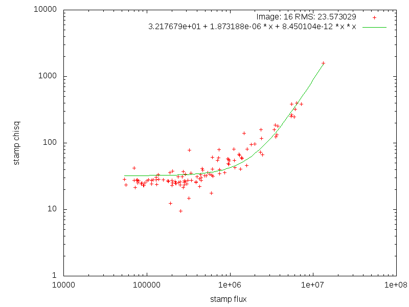
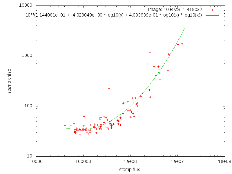
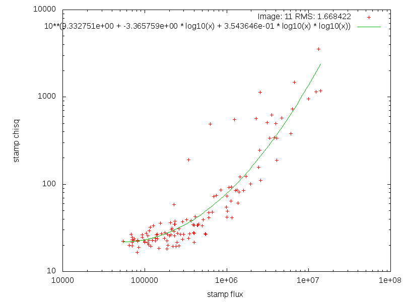
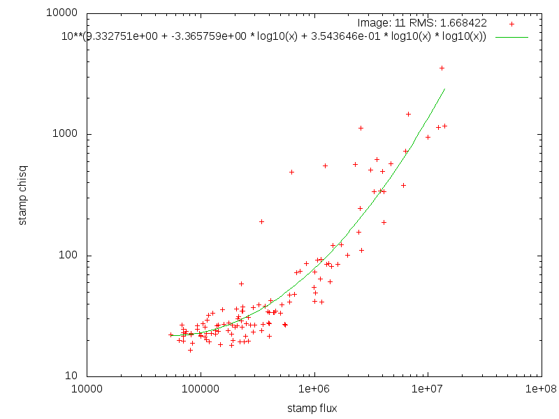
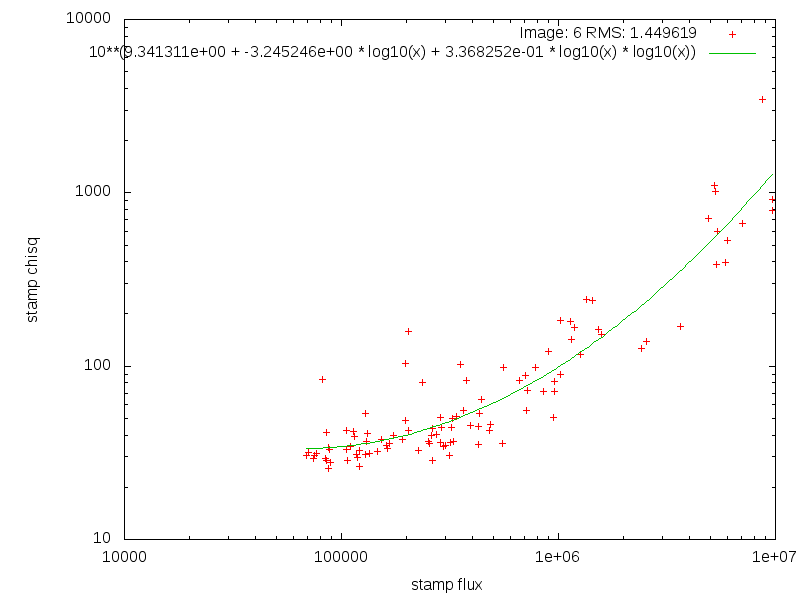
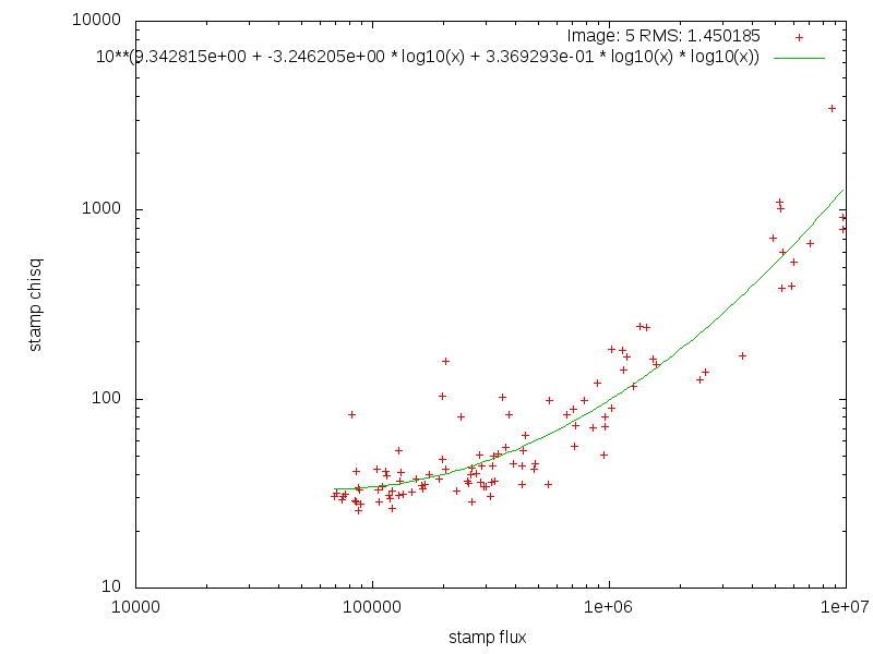
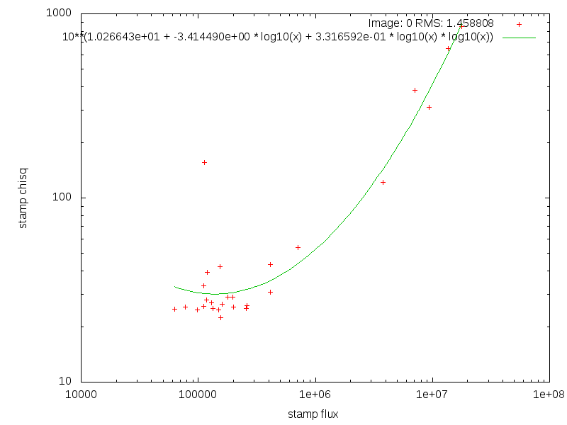
We can now plot up the data and quadratic fits to validate their quality. These plots clearly point that the large chi^2 values being used to reject input exposures at the PSF matching stage are caused by poor quadratic fits to relatively well constrained data. This supports the "by-eye" assessment that the images being rejected do not look like they should be rejected.

Comparing polynomial fits from IPP with external code, it appears that the assumption that chisq(flux) is a well-behaved quadratic function is not necessarily true. Fitting a quadratic to log10(chisq(log10(flux))) looks to provide a better fit to the data trend.

Image	Plot	Logfit Plot
0
1
2
3
4
5
6
7a
7b
8a
8b
9a
9b
10a
10b
11a
11b

2013-04-08

The new proposed algorithm for the initial ppStack FWHM cuts uses a Gaussian mixture model analysis to attempt to determine the best separation between a possible two component distribution.

• If Punimodal > 0.5 (this distribution is best described by a single Gaussian mode); limit = MAX(FWHM_i)
• Otherwise, assume two Gaussians best describe it
  • If pi1 > pi2 (the smaller FWHM group has the majority of the samples); limit = m1 + k * sigma1
  • If pi2 > pi1 (the larger FWHM group has the majority of the samples); limit = m2 + k * sigma2
  • If abs(pi1 - pi2) < separation threshold (taken as ~0.2. assume this is nearly unimodal); limit = m2 + k * sigma2
• If N <= 4; limit = MAX(FWHM_i)
• If limit > high_threshold; limit = high_threshold
• If limit < low_threshold; limit = low_threshold

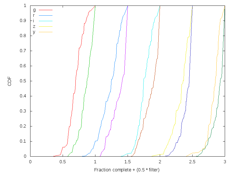
The results of this algorithm change are shows below, displaying the prior results along with this proposed change. The first figure shows the fraction of input images accepted into the stack for each filter (g,r,i,z,y). The second shows the distribution of the FWHM limits.

2013-04-04

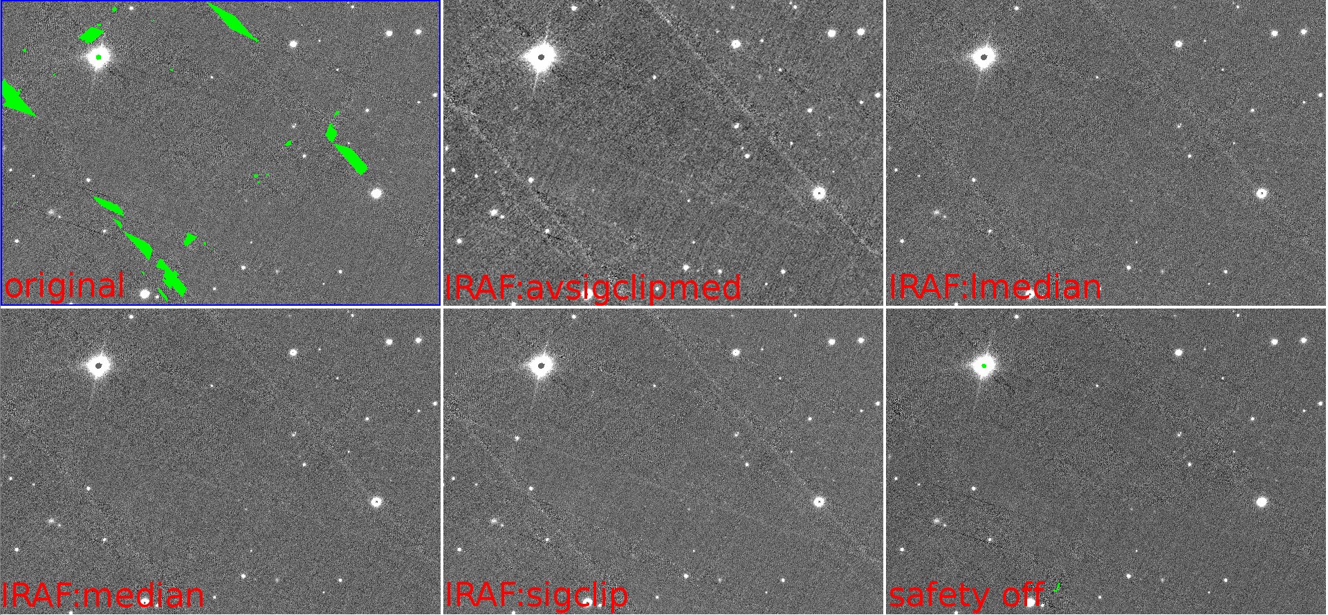
I have the first set of ppStack changes in place and merged to the trunk. This includes the fix for the PSF target that was resulting in excess detections. I have run a test on the same SAS stack that Ken and Heather were using for IRAF tests. This test has the SAFE flag set to FALSE, allowing single inputs to contribute.

2013-03-07

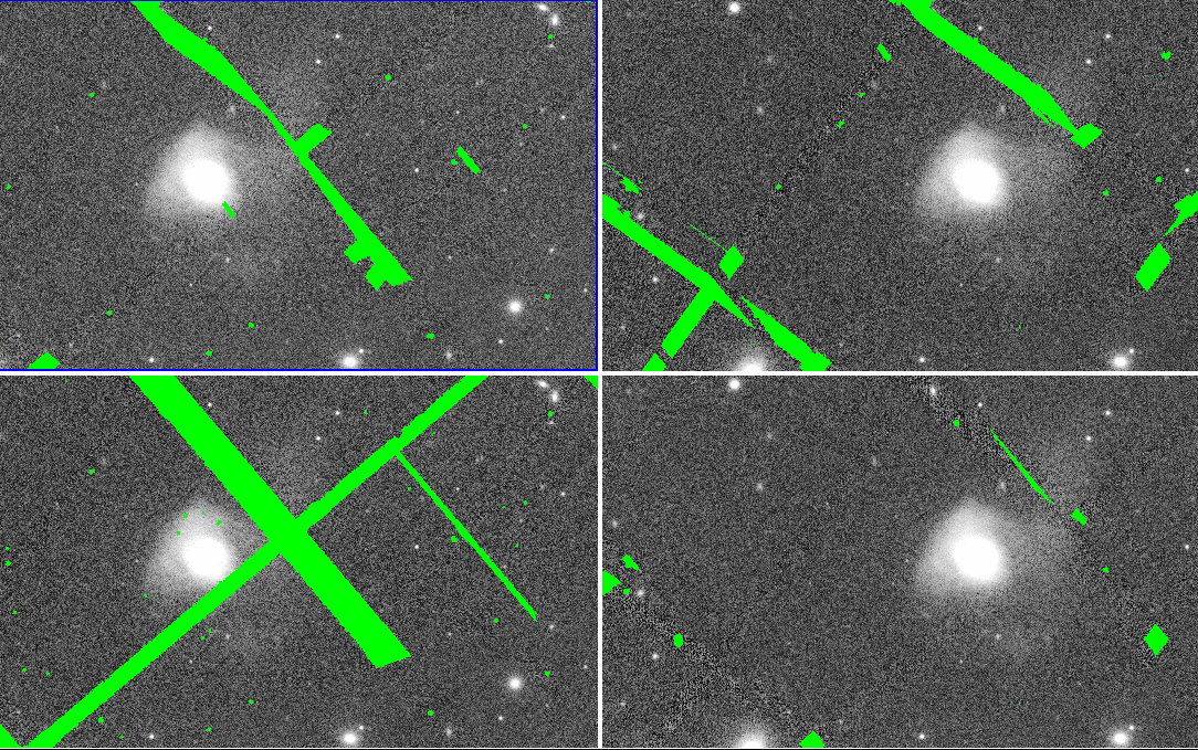
For the Arp 220 example, of the six input warps that contain the galaxies, two are excluded due to large FWHM, with another warp having a FWHM close to the hard limit of 7.5. This input was excluded in the original processing, but not in my reprocessing of the warps (FWHM for the reprocessing was 7.48). Because of this, only three (four) warps are available. We currently enforce the "safe combination" rules, which do not allow a pixel to be populated from only one input exposure. The following images show the input warps that contain Arp 220, with the top showing the reprocessed set, and the bottom showing the original warps. The red X show which inputs were excluded due to their FWHM being large. Below that is a comparison of the stacks obtained for these warps with the default combination (left panels) and with the FWHM limit set to 100, which allows all warps to contribute (right panels).