This page discusses stacks with an excess in false detections in LAP.ThreePi.20120706

2013-03-28

Using the stamp sources from yesterday's image, I've been tracing the changes in source magnitude. Something is clearly going wrong, as the sources magnitudes have unexplained offsets from the source mean values. The mean values correspond well with the measured image flux, and the source magnitudes agree with the fake magnitudes, so this unknown offset is the cause of the poor difference images/stamp matching.

x	y	frame4_mag	fake4_mag	mean match mag + 27	mean trans corr match mag + 27	options->sources->mag	source image
772.5	2688.5	-11.1479	-15.3195	-11.1882	-11.1910	-15.4301	4
984.5	2808.5	-10.9484	-15.1513	-11.0018	-11.0037	-15.2834	4
1065.5	2466.5	-11.0110	-15.1431	-11.0203	-11.0232	-15.2752	4
1202.5	2127.5	-13.6749	-14.6820	-9.5210	27.0000	-14.3078	7
1329.5	2185.5	-10.7457	-10.6698	-10.8180	-10.8166	-10.8052	2
1625.5	2484.5	-11.4295	-11.3627	-11.4733	-11.4722	-11.5002	2
1679.5	2922.5	-10.1135	-10.0500	-10.1504	-10.1497	-10.1459	2
1782.5	2532.5	-11.6375	-11.5473	-11.6697	-11.6684	-11.6654	2
2136.5	2773.5	-10.1570	-10.0263	-10.1656	-10.1650	-10.1796	2
2144.5	2449.5	-11.6187	-11.4890	-8.5305	-11.6028	-11.6344	2
2296.5	2509.5	-10.5183	-10.4174	-10.5561	-10.5551	-10.5770	2

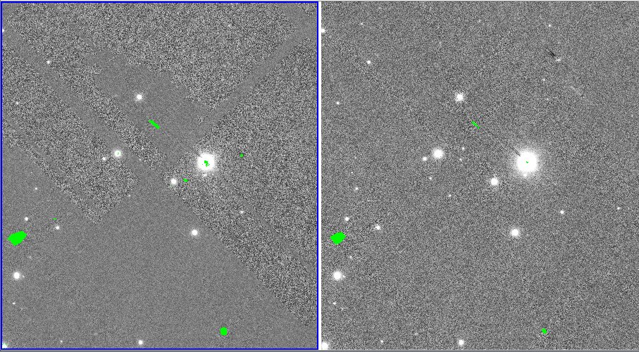
This offset (~4 mag) is similar to the magCorr values listed below. This prompted a scan of the code which led to the following conclusion: We apply a magnitude correction to the sources used to construct the fake images. However, we then compare those fake images to the convolved images that have not had a zpt/airmass/transparancy correction at all. Therefore, when magCorr is large, it seems like we introduce an arbitrary offset. I do not fully understand why input 4 shows this full effect, whereas input 2 has only a marginal shift. Regardless of this uncertainty, I ran the test stack through processing with the magCorr correction disabled. As shown in the counterpart to the image from 2013-03-27, the fake now closely matches the input convolved image. The following table also shows that im2/im1 ~ 1.0 for all stamps in this region.

x	y	image1	image2	im2/im1
772.500000	2688.500000	28861.387886	26861.103215	1.07447
984.500000	2808.500000	24030.221316	23005.069802	1.04456
1065.500000	2466.500000	25451.779205	22765.333466	1.11801
1196.500000	2121.500000	328720.052546	305653.663029	1.07547
1329.500000	2185.500000	19949.536800	18513.075711	1.07759
1625.500000	2484.500000	37385.893038	34880.027914	1.07184
1679.500000	2922.500000	11179.066752	9866.646183	1.13302
1782.500000	2532.500000	45261.595236	40720.039389	1.11153
2136.500000	2773.500000	11632.260924	10390.969721	1.11946
2144.500000	2449.500000	44486.904098	39580.071845	1.12397
2296.500000	2509.500000	16195.190695	14869.404454	1.08916

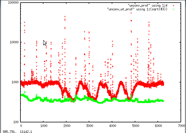
Continuing through to the output stack, the heavy mottling from before is gone, with an expected smooth noise pattern with slight bumps where the number of input frames is smaller (top panels, new unconvolved stack and variance; bottom panels, old unconvolved stack and variance). Plotting up the image and variance profiles again for this new stack (scaled by a factor of 10 to not mask out the profiles from the old stack) shows that the image and variance frame now resemble each other, so the excess detections previously found on this stack should not be an issue.

2013-03-27

This is the result of tracking down the normalization calculation in pmSubtractionCalculateNormalizationStamp. Note the position dependence of the residuals for this example exposure.

2013-03-25

Variance tracking:

Input	0	2	5	6	7	8	9	10	11
Final output variance	28931.6	27457	222888	9.29134e+06	8.36253e+06	3.59992e+06	5.38369e+06	2.93829e+06	4.33172e+06
Renormalized variance	24098.2	23265.7	210261	9.20041e+06	8.20598e+06	3.63556e+06	5.90689e+06	3.61636e+06	4.2236e+06
Pre normalized variance	19575	19701	56.523e	2717.6	2353.3	1084.4	1926.9	1061.9	1145.5
Convolved variance	8.51143e-05*	0.000105169*	54.4376	1755.02	1549.43	1069.16	1289.12	666.908	1117.07
Original variance	177.46	187.20	354.72	190.00	224.62	175.95	141.51	143.61	181.72

Starred variances are underestimates, as the convolved variance maps do not have NAN values where data is missing, but rather have 0.0. This data is therefore not excluded correctly in my statistics. In any case, it appears that the convolution process has introduced the large discrepancy in the variances. The following images show the convolved images and variance, along with the fake - convolved difference images produced by ppStack. The diff frames highlight the fact that the scaling is incredibly far off from the optimum value.

2013-03-07

Summary of photometry issues raised by Eddie

Summary of stacking coverage/completeness

2013-03-04

Updated table of values with the weight values/addVariance values:

Convolved
Input	(972,3213)	V(972,3213)	W(972,3213)	addVar(972,3213)	(884,3265)	V(884,3265)	W(884,3265)	addVar(884,3265)
5					626.727	239884.48	4.20919e-06	1
6					8819.83	22743296.0	1.05271e-07	0
7					1257.02	13702581.0	1.13473e-07	1
8	1752.842	3819864.25	2.57733e-07	1
9	1410.939	12239254.00	1.6877e-07	0	-43.029	11814249.0	1.73636e-07	0
10	-1193.50	6676459.00	3.14774e-07	1	-4040.1	6465182.50	3.11899e-07	0
11	2261.310	3833109.25	2.39817e-07	0

Unconvolved
Input	(972,3213)	V(972,3213)	W(972,3213)	addVar(972,3213)	(884,3265)	V(884,3265)	W(884,3265)	addVar(884,3265)
5					-743.98	1119270.62	4.20919e-06	1
6					-1072.73	556480.12	1.05271e-07	0
7					-1004.21	774176.12	1.13473e-07	1
8	282.286	545124.937	2.57733e-07	1
9	218.888	485149.468	1.6877e-07	0	173.61	502260.06	1.73636e-07	0
10	-932.30	589893.562	3.14774e-07	1	854.40	492724.15	3.11899e-07	0
11	-932.70	427439.906	2.39817e-07	0

2013-03-01

Manually running this example stack has clarified what the issue with the variance is. Bill was correct, it is a result of the matching chi2 and the additional variance term. Here are the fwhm, chi2, additional variance values for each unrejected input, along with the input pixel values of both the warp and variance for two positions: (972,3213) is in the "good region," where the measured stack image variance matches the value in the variance image; (884, 3265) is in the "bad region," where the observed variance is large.

Input	FWHM	chi2	Additional variance	(972,3213)	V(972,3213)	(884,3265)	V(884,3265)	directMedian(V)	weight	covarFactor	quotedMedian	renorm
0	5.332783	5395.50	4787.18					177.457	3.54363e-05	1	28139	1.090067	51.831306	56.499603
2	5.689657	5374.62	4282.85					187.196	3.43272e-05	1	29215.4	1.081804	52.073738	56.333595
5	5.963408	907.50	850.50			-13.086	346.278	354.721	4.02272e-06	1	225657	60.426430	0.940867	56.853260
6	3.478929	51509.4	54182.36			-17.9202	155.293	189.998	1.15211e-07	1	9.73308e+06	60.152260	0.995168	59.861622
7	3.615155	33226.6	33780.03	9.52773	12495.2	-16.7375	215.064	224.625	1.19095e-07	1	8.60292e+06	60.639549	0.989420	59.997963
8	4.698586	20865.3	21285.99	4.9748	186.379	15.2201	197.564	175.954	2.59256e-07	1	3.82346e+06	59.121712	0.959769	56.743206
9	5.650547	17460.7	20780.80	3.722	169.304	2.9522	145.223	141.512	1.68029e-07	1	5.59088e+06	57.258114	1.027094	58.809479
10	4.001874	17468.4	20932.79	-15.2837	158.531	14.0066	132.417	143.609	3.18491e-07	1	3.2781e+06	59.835278	1.019466	61.000050
11	5.165414	18516.5	18769.16	-16.5952	135.316	-16.5952	200.629	181.723	2.46035e-07	1	4.35814e+06	61.347172	0.916153	56.203423

The internal values for these pixels from during the rejection phase:

Input	(972,3213)	V(972,3213)	(884,3265)	V(884,3265)
5			676.53	258444.42
6			8735.83	22301894.00
7			1249.08	13243309.00
8	1752.03	3668812.75
9	1338.07	11448818.00	-47.18	10986685.00
10	-1217.08	7237640.00	-4041.17	6502667.00
11	2353.00	4089177.00

From this data, it's clear that the additional variance terms being applied to all inputs other than 5 have the effect of down-weighting those inputs. The size of this difference in variance (up to 2 orders of magnitude) means that for the regions where input 5 has data, all other inputs are effectively rejected, resulting in a scaling of only input 5. Where input 5 has no data, all inputs have approximately the same variance, and so the rejection functions normally and the result has an enhanced s/n compared to a single input.

The PSF matching can be definitively blamed for this effect by constructing the stack using "-Db CONVOLVE F", which disables the PSF matching. In this case, no additional variance is added to any input, and the output looks like what we would expect. The image below shows this, with the unconvolved stack from a standard ppStack run on the left, and the output with convolution completely removed on the right. The scales and colorbars are identical for both frames.

2013-02-27

This plot shows the measured image standard deviation (red) and the measured average variance image value (green) for each row in a 300-pixel wide vertical stripe on the stack image used as an example below. The following image shows the location of the stripe on the data and variance images. From this plot, we can see that the reason that there are so many excess detections across large regions of this image is that the variance contained in the variance image is a significant underestimate of the true image variance. Only in the areas where the image variance dips down to the excess detections drop as expected.

The reason for the discrepancy between the image and variance is not currently known.

2013-02-04

Bill Sweeney

psphotStack has found a large number of false detections in some of the stacks. This issue was discussed in December in the context of y band and changes were made to detect cases where the number of detected sources in y band was much higher than r, i, and z and turn off the feature where all forced photometry is performed in all bands for sources only detected in y.

Now that we have completed stack photometry for the most of the sky we can see how widespread the problem is.

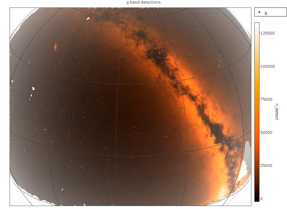
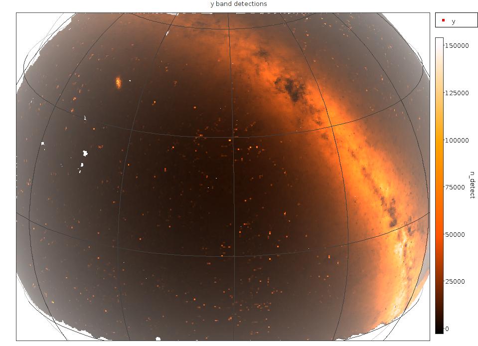
The following plot shows the number of detections per skycell as a function of RA and DEC in g and in y band. The region near the galactic plane is clearly visible as is M31. Note the various regions where the detection count is much higher than the surrounding regions. These are the skycells under discussion in this wiki page

Example y band stack 1715750 skycell.1927.074 23.1369h, 27.004d

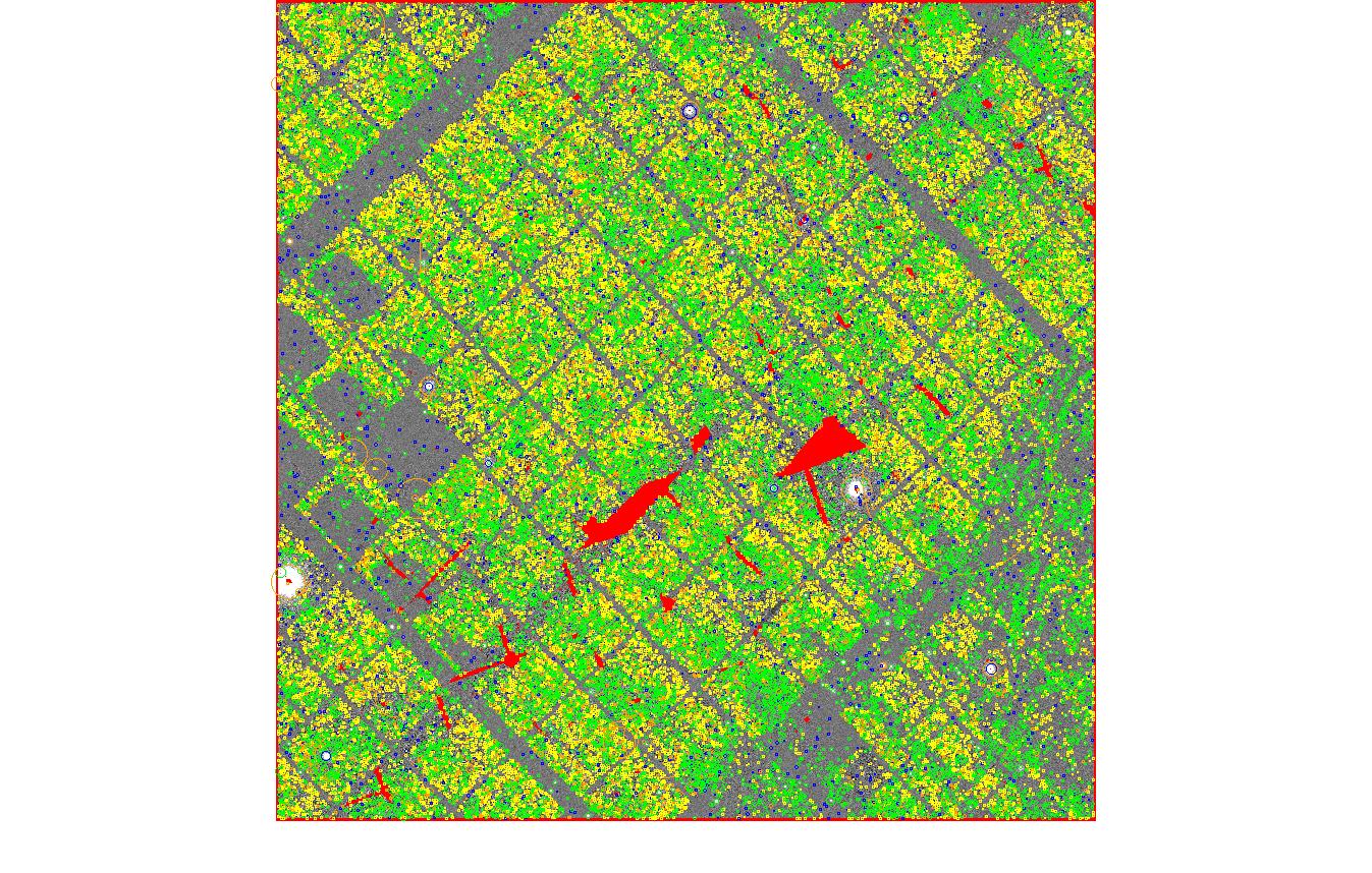
Stack_id 1715750 is an example that shows this problem. 55284 sources were detected in y band while < 6400 were detected in the stacks for the other 4 filters.

The following image shows the stack with the individual detections displayed as yellow or green circles. Note that there are areas which fall in chip and cell gaps from one or more of the inputs do not show the enhanced detections. This indicates that the phenomena is likely due to a subset of the input warps

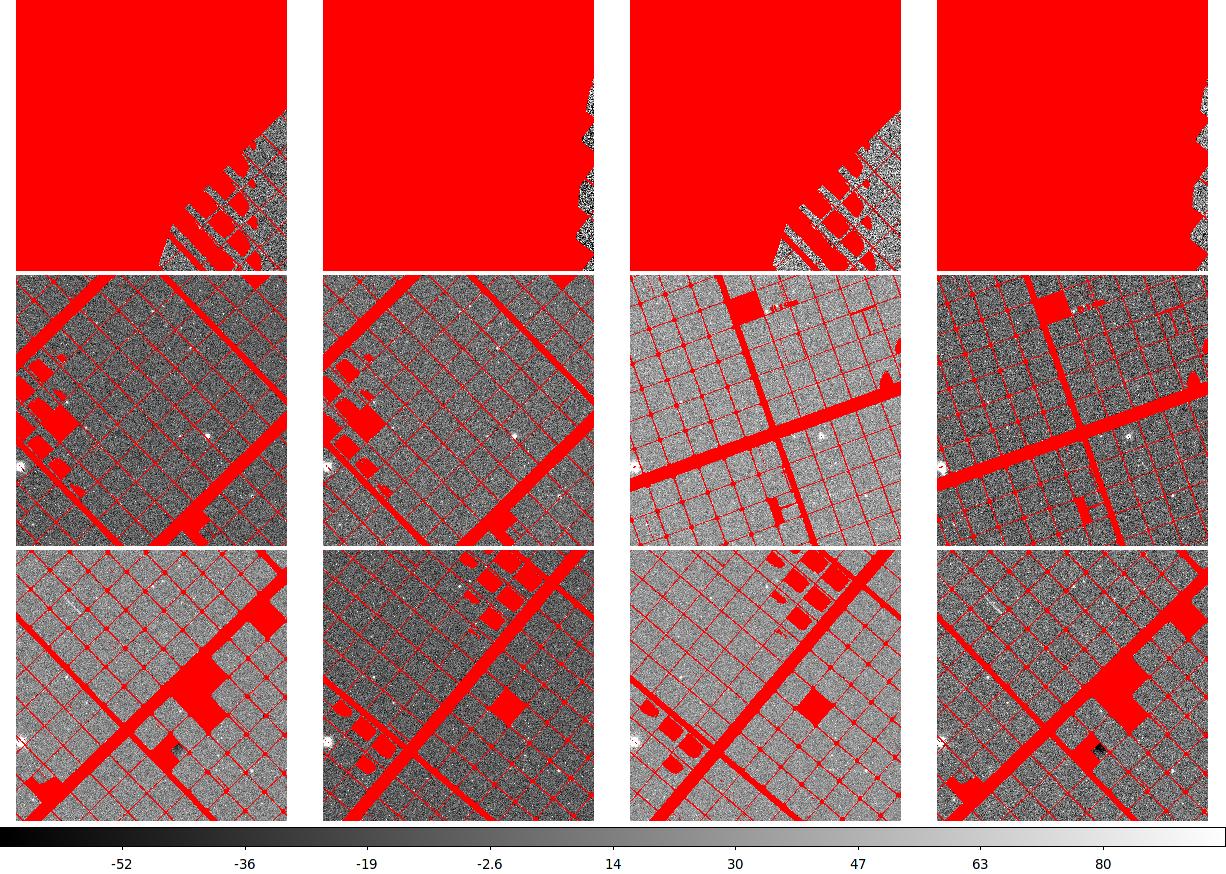
This image shows the 12 input warp images. Input 0 is on the upper left, the top row continues with inputs 1 - 3 and so on. Here we can see that the area with lower detection count matches the outline of the masked area in the fourth and fifth images. Since the fourth image was rejected it looks like the excess detections come from areas where the fifth image contributes. This is warp_id 612302. Examining the image we find obviously unusual.

Here is a copy of the log file for the stack. Input 5 has a much lower "matching chisq" and "additional variance" than the other inputs stk_1715750.log